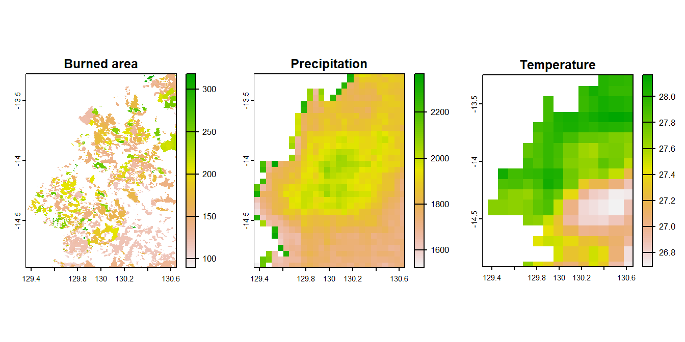
We demonstrate a spatial analysis workflow using the 2024 climate and bushfire data as an example.
We will perform spatial hot spot and cold spot analysis using the rgeoda package and conduct spatial stratified heterogeneity analysis using the GD package.
You can install the required packages using the following commands in the R console:
Figure 3.1: Maps of the 2024 climate and bushfire data
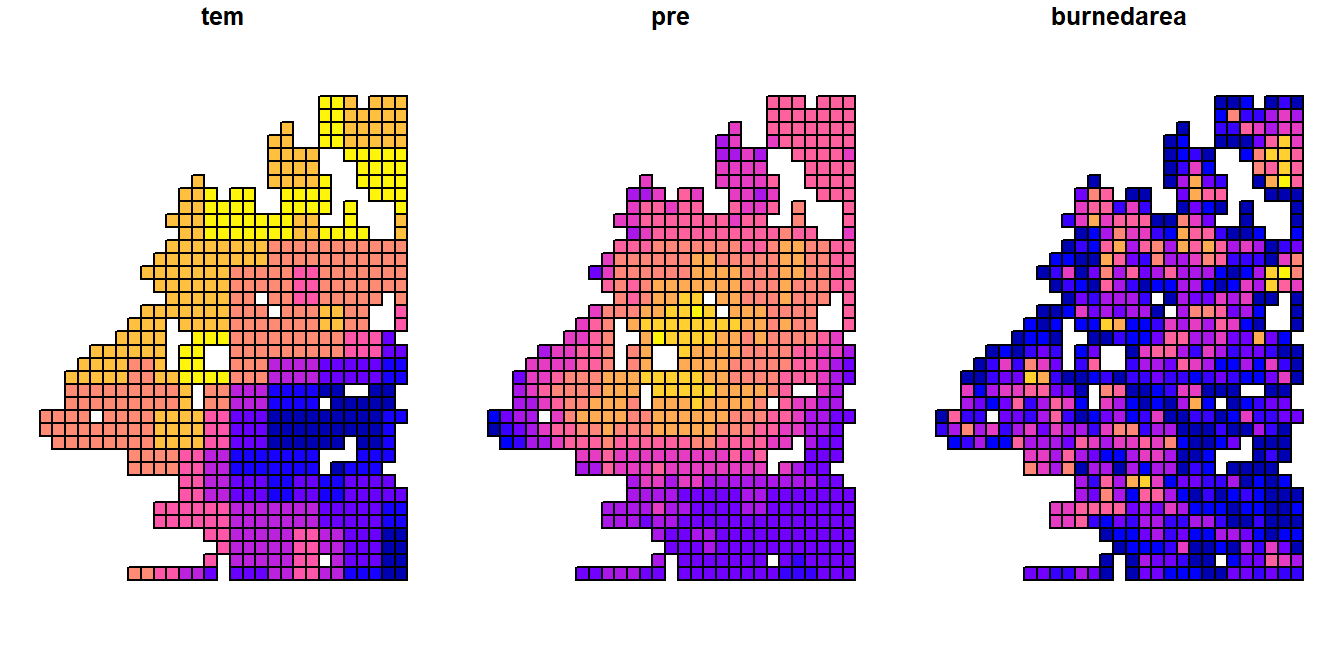
Since the row and column numbers of the three rasters are not aligned, we first convert the non-NA cells of the temperature raster into a spatial polygon format. Then, we perform zonal statistics on temperature and wildfire data, and finally, remove all NA values corresponding to the three variables.
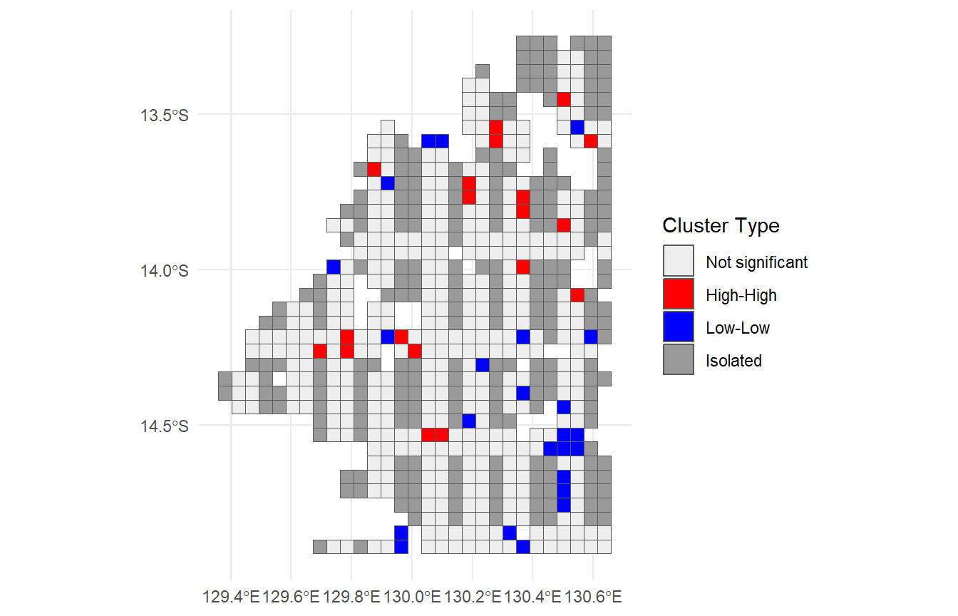
Figure 3.3: Bushfire burned area spatial hotspot analysis
3.2 Geographical detector for spatial heterogeneity and factor analysis
Aim
This step is designed to identify the climatic driving factors of bushfire burned area. We will use the GD package to analyze the power of determinant of climatic drivers on bushfire burned area based on the optimal parameter geographical detector model.
Description of steps
Load necessary libraries (sf for spatial data and gdverse for geographical detector analysis).
Read the burned area and climate data.
Run the OPGD model.
Code
library(sf)library(GD)burnedarea=read_sf('./data/3. Spatial analysis/burnedarea_2024.shp')opgd.m=gdm(burnedarea~tem+pre, continuous_variable =c("tem", "pre"), data =sf::st_drop_geometry(burnedarea), discmethod =c("equal","natural","quantile"), discitv =3:15)opgd.m# Explanatory variables include 2 continuous variables.# # optimal discretization result of tem# method : quantile# number of intervals: 13# intervals:# 26.7 26.8 27 27.2 27.3 27.5 27.7 27.7 27.7 27.8 27.9 28 28 28.2# numbers of data within intervals:# 52 47 52 47 53 47 50 49 50 50 48 50 49# # optimal discretization result of pre# method : natural# number of intervals: 14# intervals:# 1589 1650 1712 1736 1758 1787 1816 1844 1870 1896 1924 1949 1977 2011 2067# numbers of data within intervals:# 3 16 71 40 40 44 50 76 68 62 57 52 43 22# # Geographical detectors results:# # Factor detector:# variable qv sig# 1 tem 0.1301 1.79e-10# 2 pre 0.0733 2.86e-05# # Risk detector:# tem# itv meanrisk# 1 [26.69,26.8] 3730# 2 (26.8,27.02] 4871# 3 (27.02,27.2] 5984# 4 (27.2,27.33] 5647# 5 (27.33,27.51] 5514# 6 (27.51,27.66] 9252# 7 (27.66,27.69] 8948# 8 (27.69,27.74] 6647# 9 (27.74,27.83] 9489# 10 (27.83,27.91] 7340# 11 (27.91,27.96] 5083# 12 (27.96,28.02] 7738# 13 (28.02,28.16] 7136# # pre# itv meanrisk# 1 [1.59e+03,1.65e+03] 3435# 2 (1.65e+03,1.71e+03] 5166# 3 (1.71e+03,1.74e+03] 4348# 4 (1.74e+03,1.76e+03] 4829# 5 (1.76e+03,1.79e+03] 7293# 6 (1.79e+03,1.82e+03] 5739# 7 (1.82e+03,1.84e+03] 6155# 8 (1.84e+03,1.87e+03] 7578# 9 (1.87e+03,1.9e+03] 7887# 10 (1.9e+03,1.92e+03] 7212# 11 (1.92e+03,1.95e+03] 7933# 12 (1.95e+03,1.98e+03] 8390# 13 (1.98e+03,2.01e+03] 6340# 14 (2.01e+03,2.07e+03] 7009# # tem# interval [26.69,26.8] (26.8,27.02] (27.02,27.2]# 1 [26.69,26.8] <NA> <NA> <NA># 2 (26.8,27.02] N <NA> <NA># 3 (27.02,27.2] Y N <NA># 4 (27.2,27.33] Y N N# 5 (27.33,27.51] Y N N# 6 (27.51,27.66] Y Y Y# 7 (27.66,27.69] Y Y Y# 8 (27.69,27.74] Y Y N# 9 (27.74,27.83] Y Y Y# 10 (27.83,27.91] Y Y N# 11 (27.91,27.96] N N N# 12 (27.96,28.02] Y Y N# 13 (28.02,28.16] Y Y N# (27.2,27.33] (27.33,27.51] (27.51,27.66] (27.66,27.69]# 1 <NA> <NA> <NA> <NA># 2 <NA> <NA> <NA> <NA># 3 <NA> <NA> <NA> <NA># 4 <NA> <NA> <NA> <NA># 5 N <NA> <NA> <NA># 6 Y Y <NA> <NA># 7 Y Y N <NA># 8 N N Y Y# 9 Y Y N N# 10 N Y Y N# 11 N N Y Y# 12 Y Y N N# 13 N N Y N# (27.69,27.74] (27.74,27.83] (27.83,27.91] (27.91,27.96]# 1 <NA> <NA> <NA> <NA># 2 <NA> <NA> <NA> <NA># 3 <NA> <NA> <NA> <NA># 4 <NA> <NA> <NA> <NA># 5 <NA> <NA> <NA> <NA># 6 <NA> <NA> <NA> <NA># 7 <NA> <NA> <NA> <NA># 8 <NA> <NA> <NA> <NA># 9 Y <NA> <NA> <NA># 10 N Y <NA> <NA># 11 N Y Y <NA># 12 N N N Y# 13 N Y N N# (27.96,28.02] (28.02,28.16]# 1 <NA> <NA># 2 <NA> <NA># 3 <NA> <NA># 4 <NA> <NA># 5 <NA> <NA># 6 <NA> <NA># 7 <NA> <NA># 8 <NA> <NA># 9 <NA> <NA># 10 <NA> <NA># 11 <NA> <NA># 12 <NA> <NA># 13 N <NA># # pre# interval [1.59e+03,1.65e+03] (1.65e+03,1.71e+03]# 1 [1.59e+03,1.65e+03] <NA> <NA># 2 (1.65e+03,1.71e+03] N <NA># 3 (1.71e+03,1.74e+03] N N# 4 (1.74e+03,1.76e+03] N N# 5 (1.76e+03,1.79e+03] Y Y# 6 (1.79e+03,1.82e+03] N N# 7 (1.82e+03,1.84e+03] N N# 8 (1.84e+03,1.87e+03] Y Y# 9 (1.87e+03,1.9e+03] Y Y# 10 (1.9e+03,1.92e+03] Y N# 11 (1.92e+03,1.95e+03] Y Y# 12 (1.95e+03,1.98e+03] Y Y# 13 (1.98e+03,2.01e+03] N N# 14 (2.01e+03,2.07e+03] N N# (1.71e+03,1.74e+03] (1.74e+03,1.76e+03] (1.76e+03,1.79e+03]# 1 <NA> <NA> <NA># 2 <NA> <NA> <NA># 3 <NA> <NA> <NA># 4 N <NA> <NA># 5 Y Y <NA># 6 N N N# 7 Y N N# 8 Y Y N# 9 Y Y N# 10 Y Y N# 11 Y Y N# 12 Y Y N# 13 Y N N# 14 Y N N# (1.79e+03,1.82e+03] (1.82e+03,1.84e+03] (1.84e+03,1.87e+03]# 1 <NA> <NA> <NA># 2 <NA> <NA> <NA># 3 <NA> <NA> <NA># 4 <NA> <NA> <NA># 5 <NA> <NA> <NA># 6 <NA> <NA> <NA># 7 N <NA> <NA># 8 N N <NA># 9 Y N N# 10 N N N# 11 Y Y N# 12 Y Y N# 13 N N N# 14 N N N# (1.87e+03,1.9e+03] (1.9e+03,1.92e+03] (1.92e+03,1.95e+03]# 1 <NA> <NA> <NA># 2 <NA> <NA> <NA># 3 <NA> <NA> <NA># 4 <NA> <NA> <NA># 5 <NA> <NA> <NA># 6 <NA> <NA> <NA># 7 <NA> <NA> <NA># 8 <NA> <NA> <NA># 9 <NA> <NA> <NA># 10 N <NA> <NA># 11 N N <NA># 12 N N N# 13 N N N# 14 N N N# (1.95e+03,1.98e+03] (1.98e+03,2.01e+03] (2.01e+03,2.07e+03]# 1 <NA> <NA> <NA># 2 <NA> <NA> <NA># 3 <NA> <NA> <NA># 4 <NA> <NA> <NA># 5 <NA> <NA> <NA># 6 <NA> <NA> <NA># 7 <NA> <NA> <NA># 8 <NA> <NA> <NA># 9 <NA> <NA> <NA># 10 <NA> <NA> <NA># 11 <NA> <NA> <NA># 12 <NA> <NA> <NA># 13 Y <NA> <NA># 14 N N <NA># # Interaction detector:# variable tem pre# 1 tem NA NA# 2 pre 0.321 NA# # Ecological detector:# variable tem pre# 1 tem <NA> <NA># 2 pre Y <NA>
Source Code
# Spatial analysis for remote sensing dataWe demonstrate a spatial analysis workflow using the 2024 climate and bushfire data as an example.We will perform spatial hot spot and cold spot analysis using the [**rgeoda**](https://cran.r-project.org/web/packages/rgeoda/index.html) package and conduct spatial stratified heterogeneity analysis using the [**GD**](https://cran.r-project.org/web/packages/GD/vignettes/GD.html) package.You can install the required packages using the following commands in the R console:```rinstall.packages(c("sf","terra","tidyverse","rgeoda","GD","gpboost"),dep =TRUE)```Now we read the data to R and perform some basic data exploration:```{r fig-data-exploration, cache = FALSE, message = FALSE, echo=!knitr::is_latex_output()}#| fig.cap: "Maps of the 2024 climate and bushfire data"#| code-fold: true#| fig.height: 3.5library(terra)burnedarea =rast('./data/1. Data collection/BurnedArea/BurnedArea_2024.tif')burnedareapre =rast('./data/1. Data collection/Pre/Pre2024.tif')pretem =rast('./data/1. Data collection/Tem/Tem2024.tif')temoptions(terra.pal = grDevices::terrain.colors(100,rev = T))par(mfrow =c(1, 3))plot(burnedarea, main ='Burned area')plot(pre, main ='Precipitation')plot(tem, main ='Temperature')par(mfrow =c(1, 1))```Since the row and column numbers of the three rasters are not aligned, we first convert the non-NA cells of the temperature raster into a spatial polygon format. Then, we perform zonal statistics on temperature and wildfire data, and finally, remove all NA values corresponding to the three variables.```{r fig-map-sf-format, cache = FALSE, message = FALSE, echo=!knitr::is_latex_output()}#| fig.cap: "Maps of the 2024 climate and bushfire data in sf format"#| code-fold: true#| fig.height: 3.5tem.polygon = terra::as.polygons(tem,aggregate =FALSE)names(tem.polygon) ="tem"tem.polygon$pre = terra::zonal(pre,tem.polygon,fun ="mean",na.rm =TRUE)[,1]tem.polygon$burnedarea = terra::zonal(burnedarea,tem.polygon,fun ="sum",na.rm =TRUE)[,1]burnedarea.sf = sf::st_as_sf(tem.polygon) |> dplyr::filter(dplyr::if_all(1:3,\(.x) !is.na(.x)))burnedarea.sflibrary(sf)plot(burnedarea.sf)```save the data to a shapefile:```{r, eval = FALSE}#| code-fold: truesf::write_sf(burnedarea.sf,'./data/3. Spatial analysis/burnedarea_2024.shp',overwrite =TRUE)```## Spatial hotspot identification::: {.callout-tip title="Aim"}This step is designed to identify the spatial hot and cold spots of bushfire burned areas, which will be performed using the **rgeoda** package.:::::: {.callout-caution title="Description of steps"}1. Load necessary libraries (sf for spatial data, rgeoda for spatial analysis, ggplot2 for data visualization).2. Read the burned area and climate data.3. Create the spatial weight matrix.4. Run spatial hotspot analysis.5. Plot the result.:::```{r fig-spatial-hotspot, cache = FALSE, message = FALSE, echo=!knitr::is_latex_output()}#| fig.cap: "Bushfire burned area spatial hotspot analysis"#| code-fold: true#| fig.height: 4.5library(sf)library(rgeoda)library(ggplot2)burnedarea =read_sf('./data/3. Spatial analysis/burnedarea_2024.shp')queen_w =queen_weights(burnedarea)lisa =local_gstar(queen_w, burnedarea["burnedarea"])cats =lisa_clusters(lisa,cutoff =0.05)burnedarea$hcp =factor(lisa_labels(lisa)[cats +1],level =lisa_labels(lisa))p_color =lisa_colors(lisa)names(p_color) =lisa_labels(lisa)p_label =lisa_labels(lisa)[sort(unique(cats +1))]ggplot(burnedarea) +geom_sf(aes(fill = hcp)) +scale_fill_manual(values = p_color, labels = p_label) +theme_minimal() +labs(fill ="Cluster Type")```## Geographical detector for spatial heterogeneity and factor analysis::: {.callout-tip title="Aim"}This step is designed to identify the climatic driving factors of bushfire burned area. We will use the [**GD**](https://cran.r-project.org/web/packages/GD/vignettes/GD.html) package to analyze the power of determinant of climatic drivers on bushfire burned area based on the optimal parameter geographical detector model.:::::: {.callout-caution title="Description of steps"}1. Load necessary libraries (sf for spatial data and gdverse for geographical detector analysis).2. Read the burned area and climate data.3. Run the OPGD model.:::```{r fig-opgd, cache = FALSE, message = FALSE, echo=!knitr::is_latex_output()}#| fig.cap: "Climatic driving factors of bushfire burned area"#| code-fold: true#| fig.height: 8.5library(sf)library(GD)burnedarea =read_sf('./data/3. Spatial analysis/burnedarea_2024.shp')opgd.m =gdm(burnedarea~tem+pre, continuous_variable =c("tem", "pre"),data = sf::st_drop_geometry(burnedarea),discmethod =c("equal","natural","quantile"), discitv =3:15)opgd.m```