Load data and package
library(sf)
library(tidyverse)
library(gdverse)

depression = system.file('extdata/Depression.csv',package = 'gdverse') %>%
  read_csv() %>%
  st_as_sf(coords = c('X','Y'), crs = 4326)
depression
## Simple feature collection with 1072 features and 11 fields
## Geometry type: POINT
## Dimension:     XY
## Bounding box:  xmin: -83.1795 ymin: 32.11464 xmax: -78.6023 ymax: 35.17354
## Geodetic CRS:  WGS 84
## # A tibble: 1,072 × 12
##    Depression_prevelence PopulationDensity Population65 NoHealthInsurance
##  *                 <dbl>             <dbl>        <dbl>             <dbl>
##  1                  23.1              61.5         22.5              7.98
##  2                  22.8              58.3         16.8             11.0
##  3                  23.2              35.9         24.5              9.31
##  4                  21.8              76.1         21.8             13.2
##  5                  20.7              47.3         22.0             11
##  6                  21.3              32.5         19.2             13.0
##  7                  22                36.9         19.2             10.8
##  8                  21.2              61.5         15.9              8.57
##  9                  22.7              67.2         15.7             17.8
## 10                  20.6             254.          11.3             12.7
## # ℹ 1,062 more rows
## # ℹ 8 more variables: Neighbor_Disadvantage <dbl>, Beer <dbl>, MentalHealthPati <dbl>,
## #   NatureParks <dbl>, Casinos <dbl>, DrinkingPlaces <dbl>, X.HouseRent <dbl>,
## #   geometry <POINT [°]>
Spatial Autocorrelation of Depression Prevelence
here I use geocomplexity to calculate the global
Moran’s I:
set.seed(123456789)

gmi = geocomplexity::moran_test(depression)
gmi
## *** global spatial autocorrelation test| Variable | MoranI | EI | VarI | zI | pI |
|---|---|---|---|---|---|
| Depression_prevelence | 0.339557*** | -0.0009337 | 0.0003192 | 19.06 | 2.892e-81 |
| PopulationDensity | 0.365364*** | -0.0009337 | 0.0003192 | 20.5 | 1.052e-93 |
| Population65 | 0.180436*** | -0.0009337 | 0.0003192 | 10.15 | 1.641e-24 |
| NoHealthInsurance | 0.0791199*** | -0.0009337 | 0.0003192 | 4.48 | 3.724e-06 |
| Neighbor_Disadvantage | 0.113811*** | -0.0009337 | 0.0003192 | 6.422 | 6.723e-11 |
| Beer | 0.0902263*** | -0.0009337 | 0.0003192 | 5.102 | 1.68e-07 |
| MentalHealthPati | 0.19318*** | -0.0009337 | 0.0003192 | 10.86 | 8.534e-28 |
| NatureParks | 0.0895589*** | -0.0009337 | 0.0003192 | 5.065 | 2.045e-07 |
| Casinos | 0.243212*** | -0.0009337 | 0.0003192 | 13.66 | 8.28e-43 |
| DrinkingPlaces | 0.239054*** | -0.0009337 | 0.0003192 | 13.43 | 1.97e-41 |
| X.HouseRent | 0.141887*** | -0.0009337 | 0.0003192 | 7.993 | 6.562e-16 |
The global Moran’I Index of Depression Prevelence is
0.339557 and the P value is 2.892e-81, which
shows that Depression Prevelence has a moderate level of positive
spatial autocorrelation in the global scale.
OPGD modeling
depression_opgd = opgd(Depression_prevelence ~ .,
                       data = depression, cores = 12)
depression_opgd
##                 OPGD Model
## ***          Factor Detector
##
## |       variable        | Q-statistic |   P-value    |
## |:---------------------:|:-----------:|:------------:|
## | Neighbor_Disadvantage | 0.15931057  | 2.340391e-02 |
## |     Population65      | 0.11095945  | 9.999944e-01 |
## |   PopulationDensity   | 0.11065749  | 2.140000e-10 |
## |   NoHealthInsurance   | 0.08182401  | 8.340000e-10 |
## |    DrinkingPlaces     | 0.06639594  | 1.000000e+00 |
## |      NatureParks      | 0.06525932  | 1.000000e+00 |
## |      X.HouseRent      | 0.06111156  | 1.000000e+00 |
## |   MentalHealthPati    | 0.02532353  | 1.000000e+00 |
## |         Beer          | 0.02458667  | 1.000000e+00 |
## |        Casinos        | 0.01936872  | 4.363429e-01 |
You can access the detailed q statistics by
depression_opgd$factor
depression_opgd$factor
## # A tibble: 10 × 3
##    variable              `Q-statistic` `P-value`
##    <chr>                         <dbl>     <dbl>
##  1 Neighbor_Disadvantage        0.159   2.34e- 2
##  2 Population65                 0.111   1.00e+ 0
##  3 PopulationDensity            0.111   2.14e-10
##  4 NoHealthInsurance            0.0818  8.34e-10
##  5 DrinkingPlaces               0.0664  1.00e+ 0
##  6 NatureParks                  0.0653  1.00e+ 0
##  7 X.HouseRent                  0.0611  1   e+ 0
##  8 MentalHealthPati             0.0253  1   e+ 0
##  9 Beer                         0.0246  1   e+ 0
## 10 Casinos                      0.0194  4.36e- 1
Spatial Weight Matrix
SPADE explicitly considers the spatial variance by assigning the weight of the influence based on spatial distribution and also minimizes the influence of the number of levels on PD values by using the multilevel discretization and considering information loss due to discretization.
When response variable has a strong spatial dependence, maybe SPADE is a best choice.
The biggest difference between SPADE and native GD and OPGD in actual modeling is that SPADE requires a spatial weight matrix to calculate spatial variance.
In spade function, when you not provide a spatial weight
matrix, it will use 1st order inverse distance weight
by default, which can be created by
inverse_distance_weight().
coords = depression |>
  st_centroid() |>
  st_coordinates()

wt1 = inverse_distance_weight(coords[,1],coords[,2])
You can also use gravity model weight by assigning the
power parameter in inverse_distance_weight()
function.
wt2 = inverse_distance_weight(coords[,1],coords[,2],power = 2)I have also developed the sdsfun package to facilitate the construction of spatial weight matrices, which requires an input of an sf object.
wt3 = sdsfun::spdep_contiguity_swm(depression, k = 8)Or using a spatial weight matrix based on distance kernel functions.
wt4 = sdsfun::spdep_distance_swm(depression, k = 6, kernel = 'gaussian')The test of SPADE model significance in gdverse
is achieved by randomization null hypothesis use a pseudo-p value, this
calculation is very time-consuming. Default gdverse sets
the permutations parameter to 0 and does not calculate the
pseudo-p value. If you want to calculate the pseudo-p value, specify the
permutations parameter to a number such as 99,999,9999,
etc.
In the following section we will execute SPADE model using
spatial weight matrix wt1.
SPADE modeling
depression_spade = spade(Depression_prevelence ~ .,
                         data = depression,
                         wt = wt1, cores = 12)
depression_spade
## ***         Spatial Association Detector
##
## |       variable        | Q-statistic |      P-value      |
## |:---------------------:|:-----------:|:-----------------:|
## |   PopulationDensity   | 0.22350789  | No Pseudo-P Value |
## |    DrinkingPlaces     | 0.18296329  | No Pseudo-P Value |
## | Neighbor_Disadvantage | 0.17159619  | No Pseudo-P Value |
## |        Casinos        | 0.16623609  | No Pseudo-P Value |
## |     Population65      | 0.15732787  | No Pseudo-P Value |
## |      NatureParks      | 0.13953548  | No Pseudo-P Value |
## |         Beer          | 0.10609591  | No Pseudo-P Value |
## |   NoHealthInsurance   | 0.07912873  | No Pseudo-P Value |
## |   MentalHealthPati    | 0.07778826  | No Pseudo-P Value |
## |      X.HouseRent      | 0.07250500  | No Pseudo-P Value |
plot(depression_spade, slicenum = 6)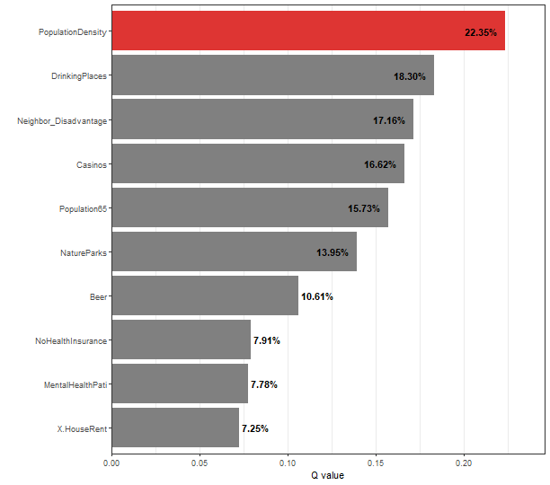
You can also access the detailed q statistics by
depression_spade$factor
depression_spade$factor
## # A tibble: 10 × 3
##    variable              `Q-statistic` `P-value`
##    <chr>                         <dbl> <chr>
##  1 PopulationDensity            0.224  No Pseudo-P Value
##  2 DrinkingPlaces               0.183  No Pseudo-P Value
##  3 Neighbor_Disadvantage        0.172  No Pseudo-P Value
##  4 Casinos                      0.166  No Pseudo-P Value
##  5 Population65                 0.157  No Pseudo-P Value
##  6 NatureParks                  0.140  No Pseudo-P Value
##  7 Beer                         0.106  No Pseudo-P Value
##  8 NoHealthInsurance            0.0791 No Pseudo-P Value
##  9 MentalHealthPati             0.0778 No Pseudo-P Value
## 10 X.HouseRent                  0.0725 No Pseudo-P Value