Optimal Parameters-based Geographical Detectors (OPGD) Model for Spatial Heterogeneity Analysis and Factor Exploration
Yongze Song
2026-02-27
Source:vignettes/GD.Rmd
GD.Rmd
Current version: GD v10.9
Citation for package GD
To cite GD R package in publications,
please use:
Song, Y., Wang, J., Ge, Y. & Xu, C. (2020) “An optimal parameters-based geographical detector model enhances geographic characteristics of explanatory variables for spatial heterogeneity analysis: Cases with different types of spatial data”, GIScience & Remote Sensing. 57(5), 593-610. doi: 10.1080/15481603.2020.1760434.
Authors’ affiliations
Dr. Yongze Song
Research interests: Spatial statistics, sustainable infrastructure
Curtin University, Australia
Email: yongze.song@curtin.edu.au
1. Introduction to GD package
1.1 The model can be used to address following issues:
Explore potential factors or explanatory variables from a spatial perspective.
Explore potential interactive impacts of geogrpahical variables.
Identify high-risk or low-risk regions from potential explanatory variables.
1.2 The GD package makes following steps fast and
easy:
It contains both supervised and unsupervised spatial data discretization methods, and the optimal spatial discretization method for continuous variables;
It contains four primary functions of geographical detectors, including factor detector, risk detector, interaction detector and ecological detector;
It can be used to compare size effects of spatial unit;
It provides diverse visualizations of spatial analysis results;
It contains detailed significance tests for spatial analysis in each step of geographical detectors.
1.3 Start from the one-step function: gdm
(Highly Recommended)
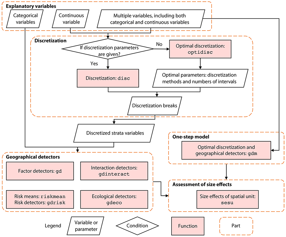
The pacakge provides a one-step function for performing optimal discretization and geographical detectors at the same time.
The output contains all data and visualization results.
## install and library the pacakge
install.packages("GD", dep = TRUE)
library(GD)

## Example 1
## NDVI: ndvi_40
## set optional parameters of optimal discretization
## optional methods: equal, natural, quantile, geometric, sd and manual
discmethod <- c("equal","natural","quantile")
discitv <- c(4:6)
## "gdm" function
## In this case, Climatezone and Mining are categorical variables,
## and Tempchange and GDP are continuous variables.
ndvigdm <- gdm(NDVIchange ~ Climatezone + Mining + Tempchange + GDP,
               continuous_variable = c("Tempchange", "GDP"),
               data = ndvi_40,
               discmethod = discmethod, discitv = discitv) # ~3s
ndvigdm
plot(ndvigdm)

## Example 2
## H1N1: h1n1_100
## set optional parameters of optimal discretization
discmethod <- c("equal","natural","quantile","geometric","sd")
discitv <- c(3:7)
continuous_variable <- colnames(h1n1_100)[-c(1,11)]
## "gdm" function
h1n1gdm <- gdm(H1N1 ~ .,
               continuous_variable = continuous_variable,
               data = h1n1_100,
               discmethod = discmethod, discitv = discitv)
h1n1gdm
plot(h1n1gdm)
1.4 Advanced models
Currently, there are the following advanced models based on spatial stratified heterogeneity.
| Model (Publication) | Description |
|---|---|
| Optimal Parameters-based Geographical Detector (OPGD) (Song et al., 2020) | OPGD is used for characterising spatial heterogeneity, identifying geographical factors and interactive impacts of factors, and estimating risks. |
| Interactive Detector for Spatial Associations (IDSA) (Song et al., 2021) | IDSA is used for estimating the power of interactive determinants (PID) from a spatial perspective. The IDSA model considers spatial heterogeneity, spatial autocorrelation, and spatial fuzzy overlay of multiple explanatory variables for calculating PID. |
| Generalized Heterogeneity Model (GHM) (Luo et al., 2023) | GHM is used for characterizing local and stratified heterogeneity within variables and to improve interpolation accuracy. |
| Geographically Optimal Zones-based Heterogeneity (GOZH) (Luo et al., 2022) | GOZH is used for identifying individual and interactive determinants of geographical attributes (e.g., global soil moisture) across a large study area. GOZH can identify optimal spatial zones and compute the maximum power of determinant (PD) values using an Ω-index. |
| Robust Geographical Detector (RGD) (Zhang et al., 2022) | RGD is used for the robust estimation of PD values. |
These methods are well supported in the gdverse package, and we welcome you to use the gdverse package we developed.
2. Geographical detector model
Spatial stratified heterogeneity can be measured using geographical detectors (Wang et al. 2010, Wang et al. 2016).
Power of determinants is computed using a \(Q\)-statistic:
\[Q=1-\displaystyle \frac{\sum_{j=1}^{M} N_{j} \sigma_{j}^2}{N \sigma^2} \]
where \(N\) and \(\sigma^2\) are the number and population variance of observations within the whole study area, and \(N_{j}\) and \(\sigma_{j}^2\) are the number and population variance of observations within the \(j\) th (\(j\)=1,…,\(M\)) sub-region of an explanatory variable.
Please note that in R environment,
sd and var functions are used for computing
sample standard deviation and sample variance. If sample
variance is used in the computation, the equation of \(Q\)-statistic can be converted to:
\[Q=1-\displaystyle \frac{\sum_{j=1}^{M} (N_{j}-1) s_{j}^2}{(N-1) s^2} \]
where \(s^2\) and \(s_{j}^2\) are sample variance of observations in the whole study area and in the \(j\) th sub-region.
Further information can be found on the manual of GD package.
More applications of geographical detectors are listed on Geodetector website.
3. Spatial data discretization
Categorical variables are required for geographical detectors, so
continuous variables should be discretized before modelling.
GD package provides two options: discretization with
given parameters, including discretization methods and numbers of
intervals, and optimal discretization with a series of optional
parameter combinations. Dataset ndvi_40 is used as an
example for explanation.
install.packages("GD")## This is GD 10.10.
##
## To cite GD in publications, please use:
##
## Song, Y., Wang, J., Ge, Y. & Xu, C. (2020) An optimal parameters-based geographical detector model enhances geographic characteristics of explanatory variables for spatial heterogeneity analysis: Cases with different types of spatial data, GIScience & Remote Sensing, 57(5), 593-610. doi: 10.1080/15481603.2020.1760434.
##
## If you find that GD runs for a long time without returning results, please try using the gdverse package we developed.
## ## NDVIchange Climatezone Mining Tempchange Precipitation GDP Popdensity
## 1 0.11599 Bwk low 0.25598 236.54 12.55 1.44957
## 2 0.01783 Bwk low 0.27341 213.55 2.69 0.80124
## 3 0.13817 Bsk low 0.30247 448.88 20.06 11.494323.1 Discretization with given parameters: disc
## discretization methods: equal, natural, quantile (default), geometric, sd and manual
ds1 <- disc(ndvi_40$Tempchange, 4)
ds1
plot(ds1)
Further information can be found on the manual of GD package.
3.2 Optimal discretization: optidisc
## set optional discretization methods and numbers of intervals
discmethod <- c("equal","natural","quantile","geometric","sd")
discitv <- c(4:7)
## optimal discretization
odc1 <- optidisc(NDVIchange ~ Tempchange, data = ndvi_40,
                 discmethod, discitv)
odc1
plot(odc1)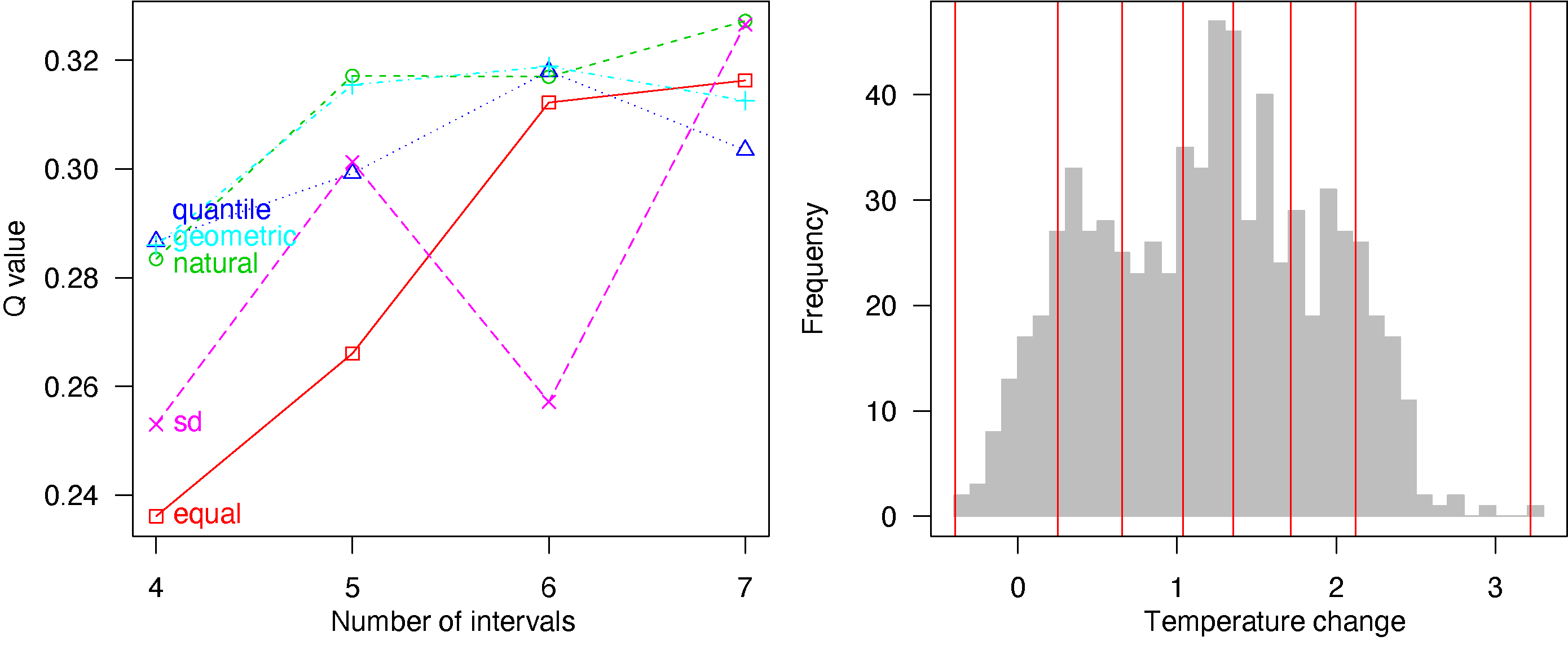
4. Geographical detectors
GD package provides two options for geographical detectors modelling:
four functions are performed step by step:
gdfor factor detector,riskmeanandgdriskfor risk detector,gdinteractfor interaction detector andgdecofor ecological detector;optimal discretization and geographical detectors are performed using a one-step function
gdm.
4.1 Factor detector: gd
## a categorical explanatory variable
g1 <- gd(NDVIchange ~ Climatezone, data = ndvi_40)
g1

## multiple categorical explanatory variables
g2 <- gd(NDVIchange ~ ., data = ndvi_40[,1:3])
g2
plot(g2)

## multiple variables including continuous variables
discmethod <- c("equal","natural","quantile","geometric","sd")
discitv <- c(3:7)
data.ndvi <- ndvi_40

data.continuous <- data.ndvi[, c(1, 4:7)]
odc1 <- optidisc(NDVIchange ~ ., data = data.continuous, discmethod, discitv) # ~14s
data.continuous <- do.call(cbind, lapply(1:4, function(x)
  data.frame(cut(data.continuous[, -1][, x], unique(odc1[[x]]$itv), include.lowest = TRUE))))
    # add stratified data to explanatory variables
data.ndvi[, 4:7] <- data.continuous

g3 <- gd(NDVIchange ~ ., data = data.ndvi)
g3
plot(g3)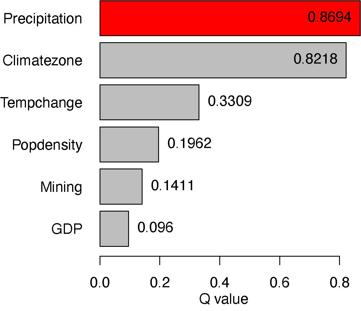
4.2 Risk detector: riskmean and
gdrisk
Risk mean values by variables:
## categorical explanatory variables
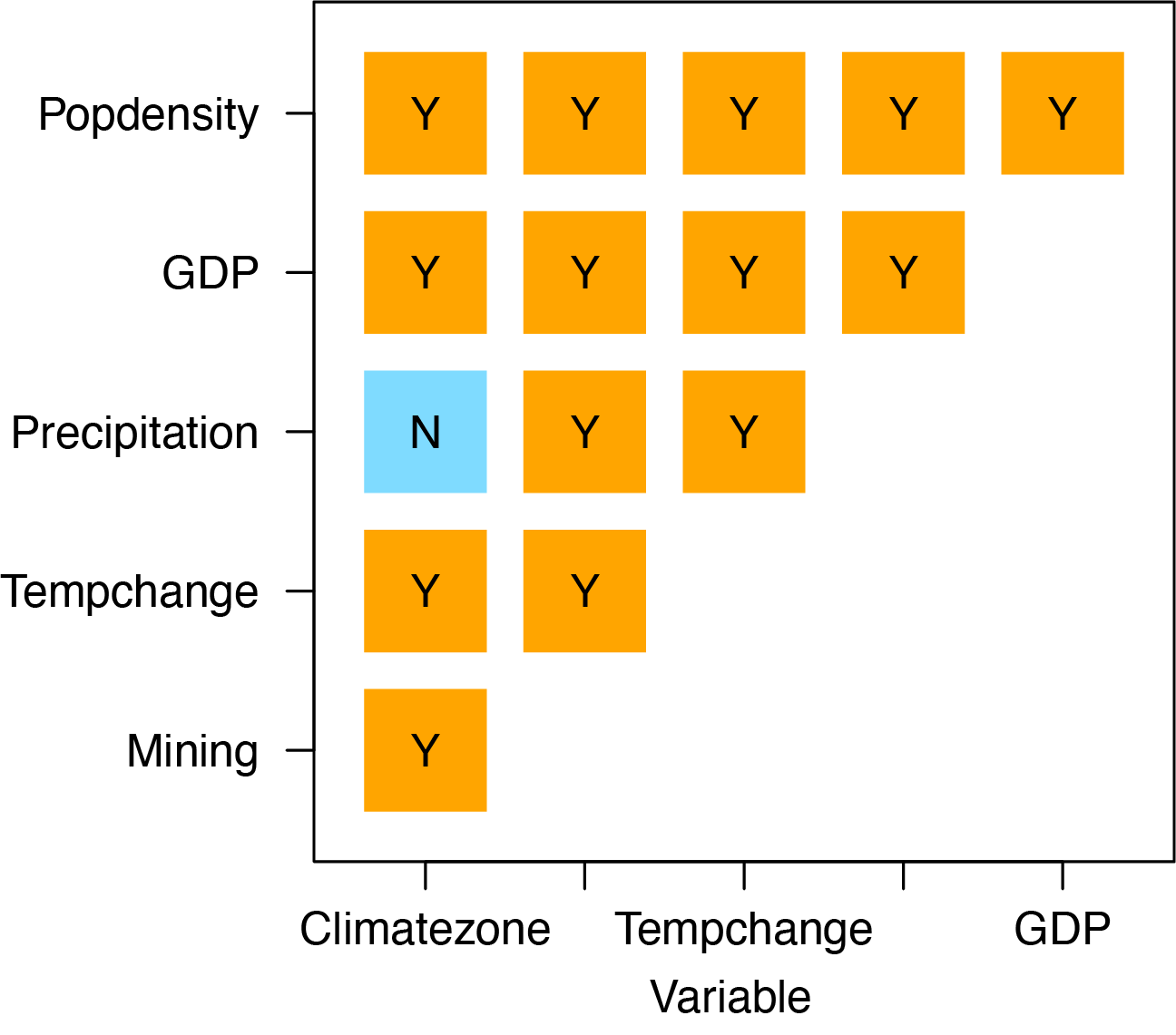
rm1 <- riskmean(NDVIchange ~ Climatezone + Mining, data = ndvi_40)
rm1
plot(rm1)
## multiple variables inclusing continuous variables
rm2 <- riskmean(NDVIchange ~ ., data = data.ndvi)
rm2
plot(rm2)
Risk matrix:
## categorical explanatory variables
gr1 <- gdrisk(NDVIchange ~ Climatezone + Mining, data = ndvi_40)
gr1
plot(gr1)
## multiple variables inclusing continuous variables
gr2 <- gdrisk(NDVIchange ~ ., data = data.ndvi)
gr2
plot(gr2)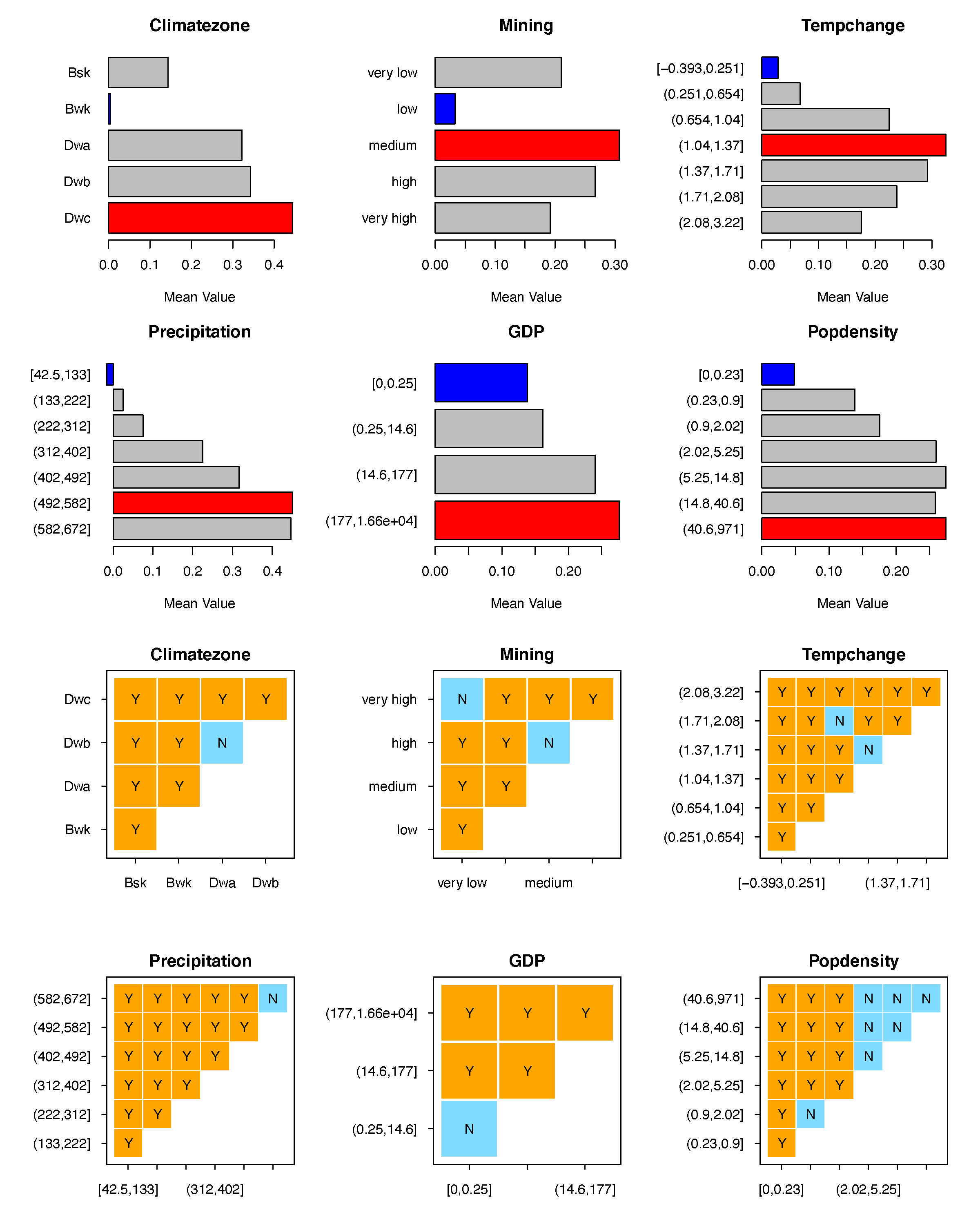
4.3 Interaction detector: gdinteract
## categorical explanatory variables
gi1 <- gdinteract(NDVIchange ~ Climatezone + Mining, data = ndvi_40)
gi1
## multiple variables inclusing continuous variables
gi2 <- gdinteract(NDVIchange ~ ., data = data.ndvi)
gi2
plot(gi2)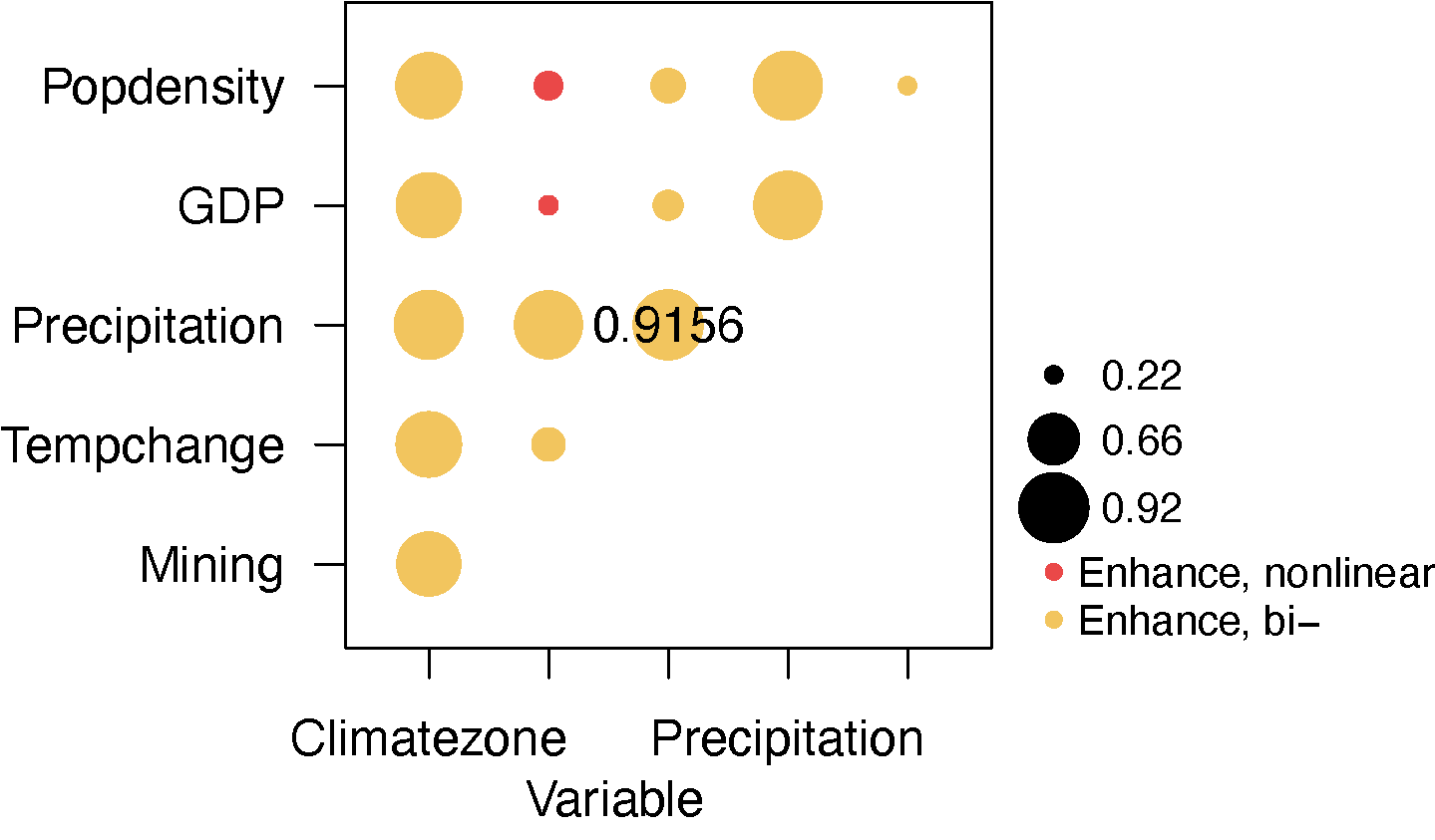
5. Comparison of size effects of spatial unit
ndvilist <- list(ndvi_20, ndvi_30, ndvi_40, ndvi_50)
su <- c(20,30,40,50) ## sizes of spatial units
## "gdm" function
gdlist <- lapply(ndvilist, function(x){
  gdm(NDVIchange ~ Climatezone + Mining + Tempchange + GDP,
      continuous_variable = c("Tempchange", "GDP"),
      data = x, discmethod = "quantile", discitv = 6)
})
sesu(gdlist, su) ## size effects of spatial units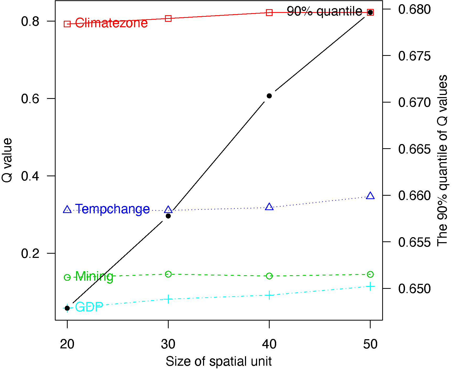
Reference
Song, Y., Wang, J.F., Ge, Y., et al. An optimal parameters-based geographical detector model enhances geographic characteristics of explanatory variables for spatial heterogeneity analysis: cases with different types of spatial data. GIScience & Remote Sensing, 2020. 57(5): 593-610. doi: 10.1080/15481603.2020.1760434.
Wang, J. F., Li, X. H., Christakos, G., Liao, Y. L., et al. Geographical detectors‐based health risk assessment and its application in the neural tube defects study of the Heshun Region, China. International Journal of Geographical Information Science, 2010. 24(1), 107-127. doi: 10.1080/13658810802443457.
Wang, J. F., Zhang, T. L., & Fu, B. J. A measure of spatial stratified heterogeneity. Ecological indicators, 2016. 67, 250-256. doi: 10.1016/j.ecolind.2016.02.052.
Luo., P., Song, Y., Zhu, D., Cheng, J., & Meng, L. A generalized heterogeneity model for spatial interpolation. International Journal of Geographical Information Science. 2023, 37(3): 634-659. doi: 10.1080/13658816.2022.2147530.
Guo, J., Wang, J., Xu, C., & Song, Y. Modeling of spatial stratified heterogeneity. GIScience & Remote Sensing, 2020. 59(1), 1660-1677. doi: 10.1080/15481603.2022.2126375.
Song, Y., Wu, P. An interactive detector for spatial associations. International Journal of Geographical Information Science, 2021. doi: 10.1080/13658816.2021.1882680.
Song, Y., Wright, G., Wu, P., Thatcher, D., et al. Segment-Based Spatial Analysis for Assessing Road Infrastructure Performance Using Monitoring Observations and Remote Sensing Data. Remote Sensing, 2018. 10(11): 1696. doi: 10.3390/rs10111696.
Luo, P., Song, Y., Huang, X., Ma, H., et al. Identifying determinants of spatio-temporal disparities in soil moisture of the Northern Hemisphere using a geographically optimal zones-based heterogeneity model. ISPRS Journal of Photogrammetry and Remote Sensing, 2022. 185, 111-128. doi: 10.1016/j.isprsjprs.2022.01.009.
Zhang, Z., Song, Y., & Wu, P. Robust geographical detector. International Journal of Applied Earth Observation and Geoinformation, 2022. 109, 102782. doi: 10.1016/j.jag.2022.102782.
Song, Y., Wu, P., Gilmore, D., et al. A Spatial Heterogeneity-Based Segmentation Model for Analyzing Road Deterioration Network Data in Multi-Scale Infrastructure Systems. IEEE Transactions on Intelligent Transportation Systems, 2020. doi: 10.1109/TITS.2020.3001193.
Luo, P., Song, Y. Wu, P. Spatial disparities in trade-offs: economic and environmental impacts of road infrastructure on continental level. GIScience & Remote Sensing, 2021. doi: 10.1080/15481603.2021.1947624.
Zhang, Z., Song, Y., Archer, N. and Wu, P. Spatial disparity of urban performance from a scaling perspective: a study of industrial features associated with economy, infrastructure, and innovation. GIScience & Remote Sensing. 2023. 60(1), p.2167567. doi: 10.1080/15481603.2023.2167567.
