geocomplexity for spatial vector data based on geographical similarity

This function calculates geocomplexity for in spatial vector data based on geographical similarity.

Usage

geocs_vector(
  sfj,
  wt = NULL,
  method = "spvar",
  similarity = 1,
  normalize = TRUE,
  returnsf = TRUE
)

Arguments

sfj

An sf object or spatial vector object that can be converted to sf by sf::st_as_sf().

wt

(optional) Spatial weight matrix. Must be a matrix class. If wt is not provided, geocomplexity will use a first-order inverse distance weight matrix via sdsfun::inverse_distance_swm() function.

method

(optional) When method is spvar, variation of the similarity vector is represented using spatial variance, otherwise shannon information entropy is used. Default is spvar.

similarity

(optional) When similarity is 1, the similarity is calculated using geographical configuration similarity, otherwise the cosine similarity is calculated. Default is 1.

normalize

(optional) Whether to further normalizes the calculated geocomplexity. Default is TRUE.

returnsf

(optional) When returnsf is TRUE, return an sf object, otherwise a tibble. Default is TRUE.

Value

A tibble (returnsf is FALSE) or an sf object (returnsf is TRUE)

Examples

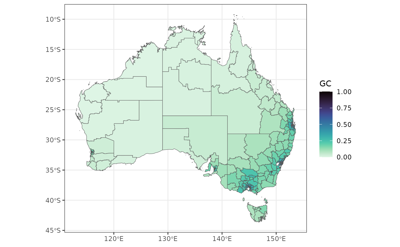
econineq = sf::read_sf(system.file('extdata/econineq.gpkg',package = 'geocomplexity'))
gc = geocs_vector(dplyr::select(econineq,-Gini))
gc
#> Simple feature collection with 333 features and 1 field
#> Geometry type: MULTIPOLYGON
#> Dimension:     XY
#> Bounding box:  xmin: 112.9211 ymin: -43.63311 xmax: 153.6299 ymax: -9.223927
#> Geodetic CRS:  GDA94
#> # A tibble: 333 × 2
#>       GC                                                                geometry
#>    <dbl>                                                      <MULTIPOLYGON [°]>
#>  1 0.210 (((149.979 -35.50246, 149.9774 -35.49025, 149.9987 -35.47874, 150.0059…
#>  2 0.155 (((148.8041 -35.71402, 148.782 -35.73665, 148.7666 -35.70281, 148.7535…
#>  3 0.147 (((150.3754 -35.56524, 150.3725 -35.55018, 150.36 -35.53485, 150.2819 …
#>  4 0.213 (((149.0114 -33.93276, 149.0057 -33.94396, 149.013 -33.96863, 149.0114…
#>  5 0.184 (((147.7137 -34.16162, 147.7126 -34.17681, 147.728 -34.18633, 147.7443…
#>  6 0.353 (((151.485 -33.39868, 151.4645 -33.39985, 151.4539 -33.37713, 151.4415…
#>  7 0.307 (((151.485 -33.39868, 151.4839 -33.38366, 151.5049 -33.35415, 151.499 …
#>  8 0.214 (((149.323 -33.05916, 149.3147 -33.10072, 149.3226 -33.1168, 149.3171 …
#>  9 0.133 (((149.1264 -33.86642, 149.1349 -33.85089, 149.1314 -33.83058, 149.115…
#> 10 0.180 (((150.5587 -32.75774, 150.5411 -32.75426, 150.527 -32.75969, 150.5182…
#> # ℹ 323 more rows

library(ggplot2)
library(viridis)
ggplot(gc) +
   geom_sf(aes(fill = GC)) +
   scale_fill_viridis(option = "mako", direction = -1) +
   theme_bw()