geocomplexity for spatial vector data based on spatial dependence

This function calculates geocomplexity for spatial vector data based on spatial dependence.

Usage

geocd_vector(
  sfj,
  wt = NULL,
  method = "moran",
  normalize = TRUE,
  returnsf = TRUE
)

Arguments

sfj: An sf object or spatial vector object that can be converted to sf by sf::st_as_sf().
wt: (optional) Spatial weight matrix. Must be a matrix class.
method: (optional) In instances where the method is moran, geocomplexity is determined using local moran measure method. Conversely, when the method is spvar, the spatial variance of attribute data serves to characterize geocomplexity. For all other methods, the shannon information entropy of attribute data is employed to represent geocomplexity. The selection of the method can be made from any one of the three options: moran, spvar or entropy. Default is moran.
normalize: (optional) Whether to further normalizes the calculated geocomplexity. Default is TRUE.
returnsf: (optional) When returnsf is TRUE, return an sf object, otherwise a tibble. Default is TRUE.

Value

A tibble (returnsf is FALSE) or an sf object (returnsf is TRUE)

Note

If wt is not provided, for polygon vector data, geocomplexity will use a first-order queen adjacency binary matrix; for point vector data, the six nearest points are used as adjacency objects to generate an adjacency binary matrix.

Examples

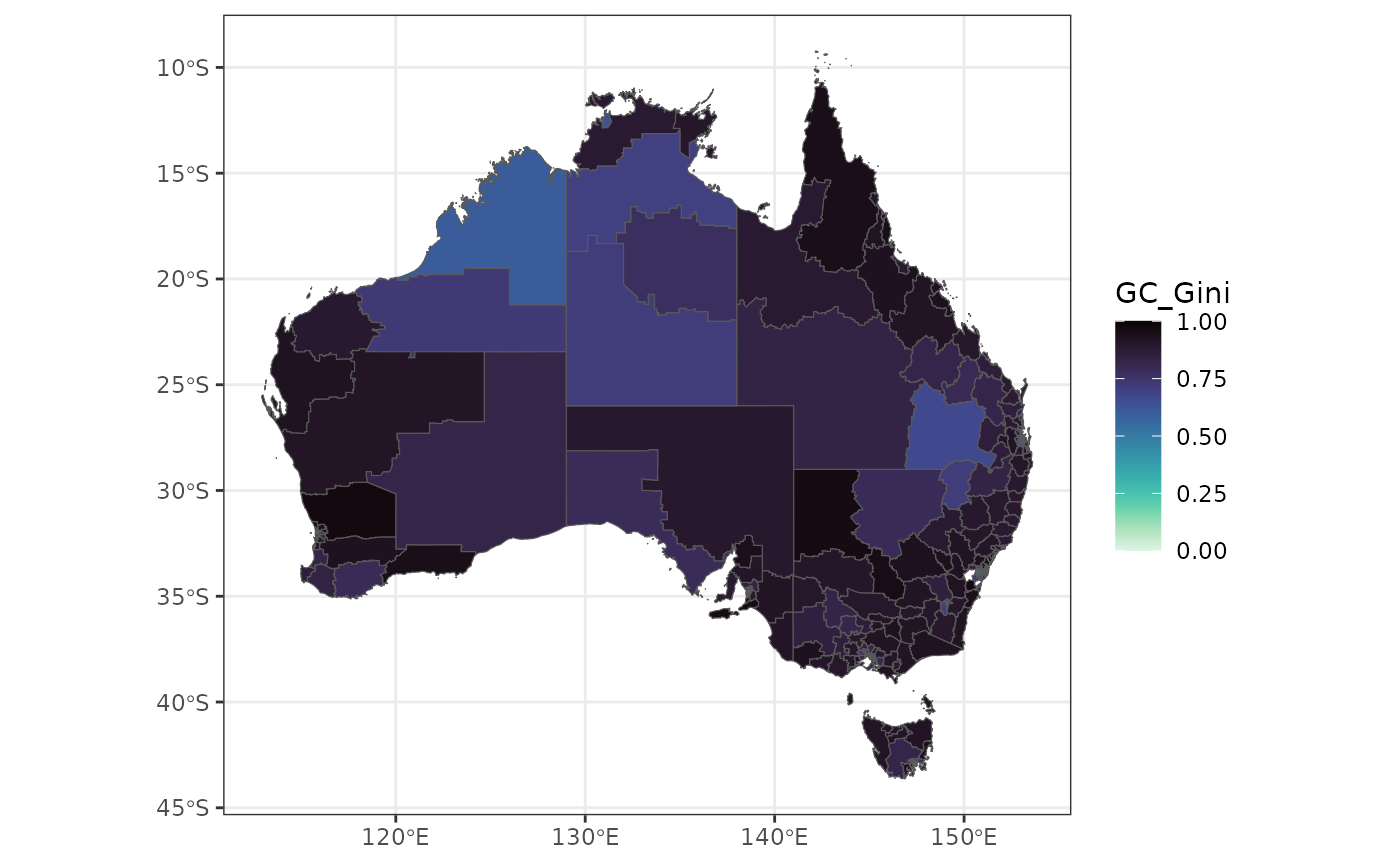
econineq = sf::read_sf(system.file('extdata/econineq.gpkg',package = 'geocomplexity'))
gc = geocd_vector(econineq)
gc
#> Simple feature collection with 333 features and 9 fields
#> Geometry type: MULTIPOLYGON
#> Dimension:     XY
#> Bounding box:  xmin: 112.9211 ymin: -43.63311 xmax: 153.6299 ymax: -9.223927
#> Geodetic CRS:  GDA94
#> # A tibble: 333 × 10
#>    GC_Gini GC_Induscale GC_IT GC_Income GC_Sexrat GC_Houseown GC_Indemp
#>      <dbl>        <dbl> <dbl>     <dbl>     <dbl>       <dbl>     <dbl>
#>  1   0.899        0.922 0.945     0.952     0.845       0.906     0.858
#>  2   0.895        0.919 0.849     0.925     0.770       0.825     0.853
#>  3   0.922        0.919 0.861     0.914     0.729       0.759     0.888
#>  4   0.921        0.919 0.834     0.949     0.775       0.807     0.892
#>  5   0.850        0.924 0.830     0.930     0.778       0.889     0.863
#>  6   0.944        0.920 0.873     0.956     0.782       0.856     0.865
#>  7   0.910        0.921 0.891     0.957     0.799       0.865     0.809
#>  8   0.924        0.919 0.817     0.938     0.810       0.834     0.910
#>  9   0.929        0.919 0.663     0.901     0.768       0.837     0.911
#> 10   0.918        0.919 0.841     0.957     0.758       0.863     0.927
#> # ℹ 323 more rows
#> # ℹ 3 more variables: GC_Indcom <dbl>, GC_Hiedu <dbl>,
#> #   geometry <MULTIPOLYGON [°]>

library(ggplot2)
library(viridis)
#> Loading required package: viridisLite
ggplot(gc) +
   geom_sf(aes(fill = GC_Gini)) +
   scale_fill_viridis(option = "mako", direction = -1) +
   theme_bw()