function for the best kappa parameter

Computationally optimized function for determining the best kappa parameter for the optimal similarity

Usage

gos_bestkappa(
  formula,
  data = NULL,
  kappa = seq(0.05, 1, 0.05),
  nrepeat = 10,
  nsplit = 0.5,
  cores = 1
)

Arguments

formula

A formula of GOS model.

data

A data.frame or tibble of observation data.

kappa

(optional) A numeric value of the percentage of observation locations with high similarity to a prediction location. \(kappa = 1 - tau\), where tau is the probability parameter in quantile operator. kappa is 0.25 means that 25% of observations with high similarity to a prediction location are used for modelling.

nrepeat

(optional) A numeric value of the number of cross-validation training times. The default value is 10.

nsplit

(optional) The sample training set segmentation ratio,which in (0,1). Default is 0.5.

cores

(optional) Positive integer. If cores > 1, a parallel package cluster with that many cores is created and used. You can also supply a cluster object. Default is 1.

Value

A list of the result of the best kappa and the computation process curve.

bestkappa

the result of best kappa

cvrmse

all RMSE calculations during cross-validation

cvmean

the average RMSE corresponding to different kappa in the cross-validation process

plot

the plot of rmse changes corresponding to different kappa

References

Song, Y. (2022). Geographically Optimal Similarity. Mathematical Geosciences. doi: 10.1007/s11004-022-10036-8.

Examples

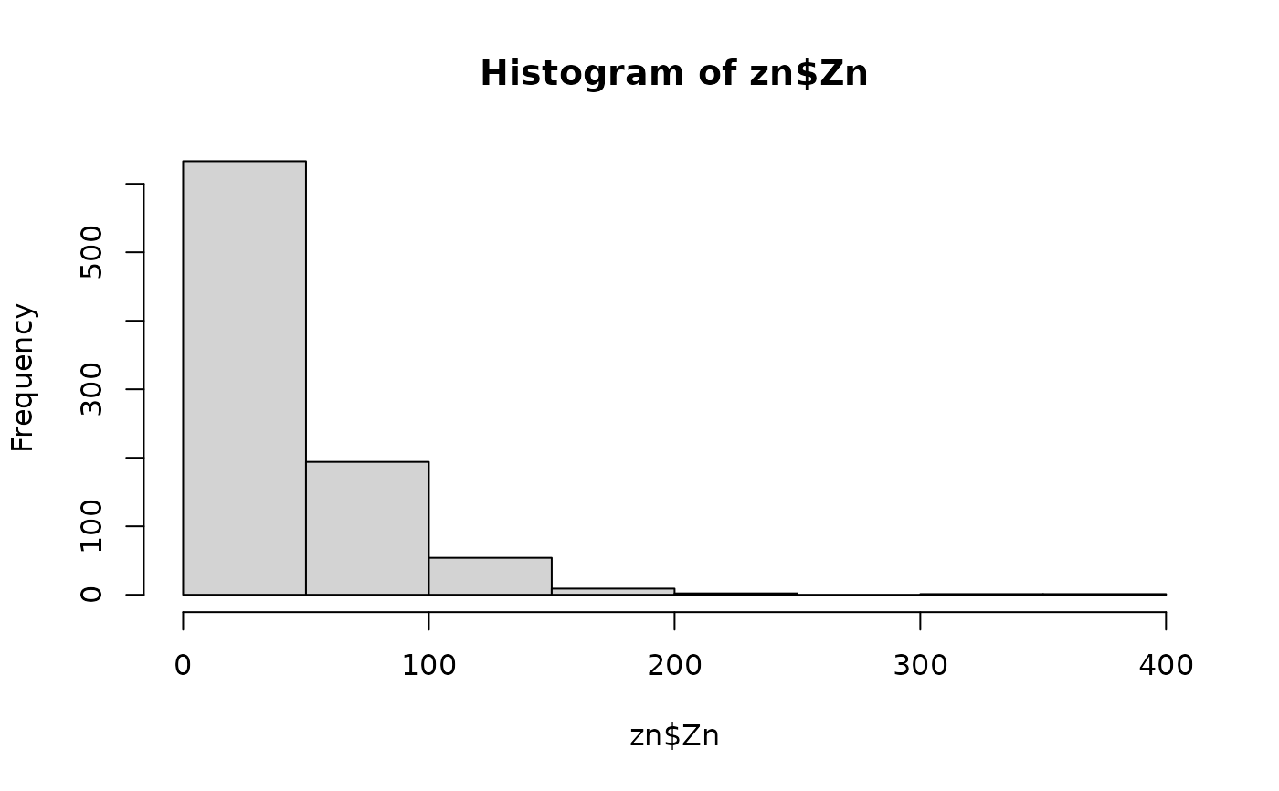
data("zn")
# log-transformation
hist(zn$Zn)

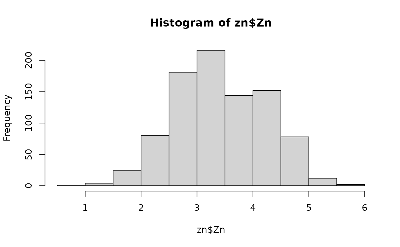
zn$Zn <- log(zn$Zn)
hist(zn$Zn)
# remove outliers
k <- removeoutlier(zn$Zn, coef = 2.5)
#> Remove 9 outlier(s)
dt <- zn[-k,]
# determine the best kappa
system.time({
b1 <- gos_bestkappa(Zn ~ Slope + Water + NDVI  + SOC + pH + Road + Mine,
                    data = dt,
                    kappa = c(0.01, 0.1, 1),
                    nrepeat = 1,
                    cores = 1)
})

#>    user  system elapsed 
#>   1.279   0.003   1.283 
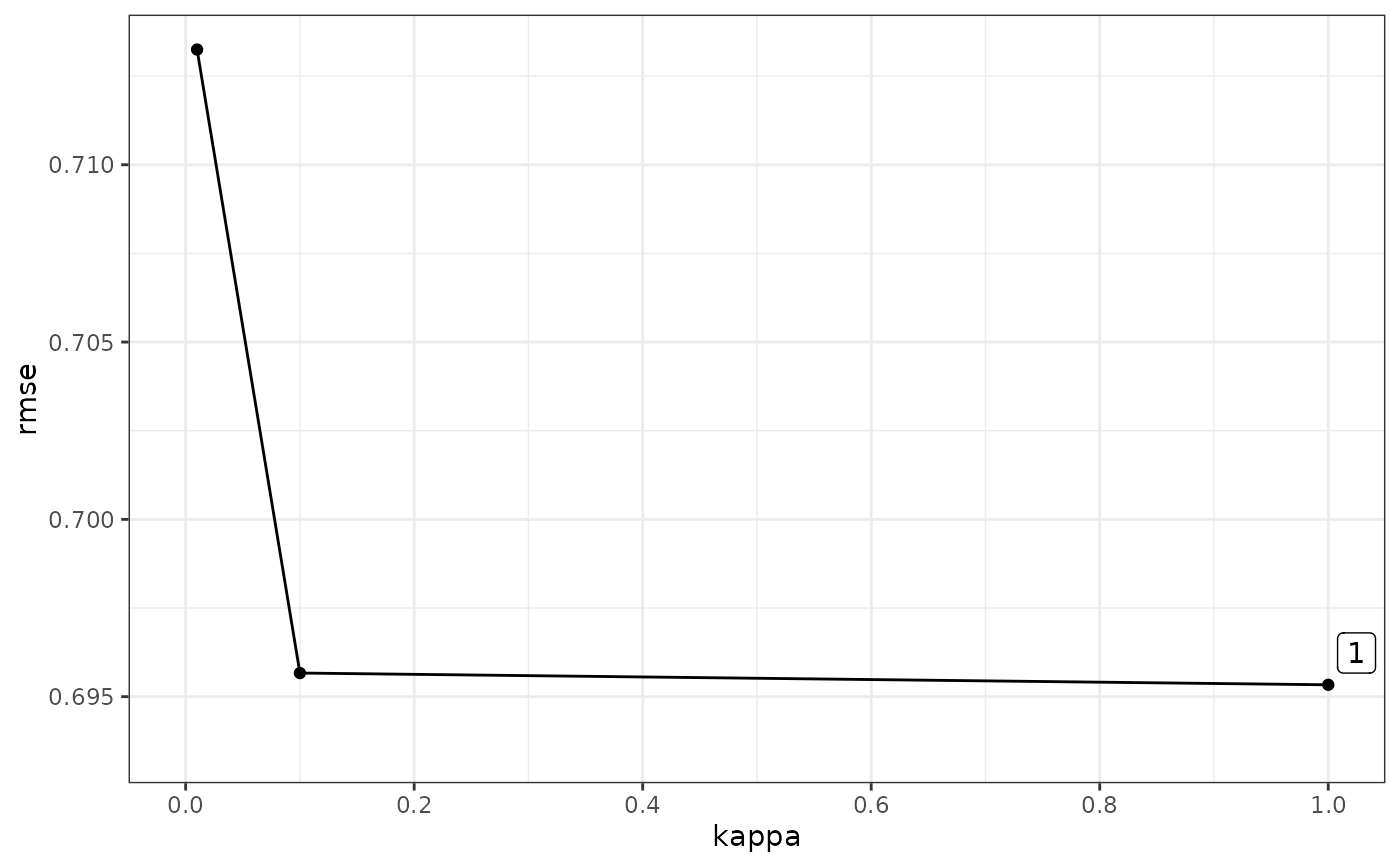
b1$bestkappa
#> [1] 1
b1$plot