geographically optimal similarity — gos • geosimilarity

Computationally optimized function for geographically optimal similarity (GOS) model

Usage

gos(formula, data = NULL, newdata = NULL, kappa = 0.25, cores = 1)

Arguments

formula: A formula of GOS model.
data: A data.frame or tibble of observation data.
newdata: A data.frame or tibble of prediction variables data.
kappa: (optional) A numeric value of the percentage of observation locations with high similarity to a prediction location. \(kappa = 1 - tau\), where tau is the probability parameter in quantile operator. The default kappa is 0.25, meaning that 25% of observations with high similarity to a prediction location are used for modelling.
cores: (optional) Positive integer. If cores > 1, a parallel package cluster with that many cores is created and used. You can also supply a cluster object. Default is 1.

Value

A tibble made up of predictions and uncertainties.

pred: GOS model prediction results
uncertainty90: uncertainty under 0.9 quantile
uncertainty95: uncertainty under 0.95 quantile
uncertainty99: uncertainty under 0.99 quantile
uncertainty99.5: uncertainty under 0.995 quantile
uncertainty99.9: uncertainty under 0.999 quantile
uncertainty100: uncertainty under 1 quantile

References

Song, Y. (2022). Geographically Optimal Similarity. Mathematical Geosciences. doi: 10.1007/s11004-022-10036-8.

Examples

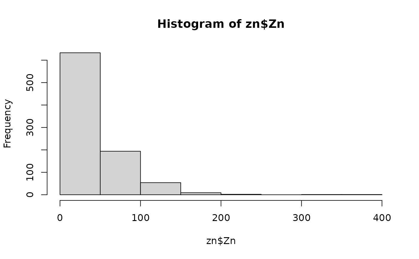
data("zn")
# log-transformation
hist(zn$Zn)

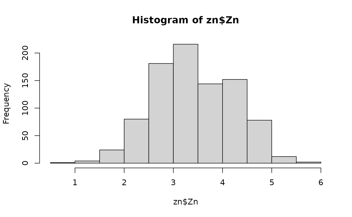
zn$Zn <- log(zn$Zn)
hist(zn$Zn)

# remove outliers
k <- removeoutlier(zn$Zn, coef = 2.5)
#> Remove 9 outlier(s)
dt <- zn[-k,]
# split data for validation: 70% training; 30% testing
split <- sample(1:nrow(dt), round(nrow(dt)*0.7))
train <- dt[split,]
test <- dt[-split,]
system.time({
g1 <- gos(Zn ~ Slope + Water + NDVI  + SOC + pH + Road + Mine,
          data = train, newdata = test, kappa = 0.25, cores = 1)
})
#>    user  system elapsed 
#>   0.321   0.018   0.338 
test$pred <- g1$pred
plot(test$Zn, test$pred)

cor(test$Zn, test$pred)
#> [1] 0.494374